40 excel data labels above bar

Solved: data labels not showing- options? - Power BI I have a bar chart and the data labels do not show on two of the three bars. It appears to be due to the bars being closer together, is there anyway to adjust the spacing or force the labels to appear above and or below? Solved! Go to Solution. Labels: Labels: Need Help; Message 1 of 7 9,971 Views 0 Reply. 1 ACCEPTED SOLUTION v-diye-msft ... Excel, giving data labels to only the top/bottom X% values 1) Create a data set next to your original series column with only the values you want labels for (again, this can be formula driven to only select the top / bottom n values). See column D below. 2) Add this data series to the chart and show the data labels. 3) Set the line color to No Line, so that it does not appear! 4) Volia! See Below! Share

Data labels on the outside end of error bars without overlapping? The easiest way to do this is to simply add 'data labels' and then replace the numeric value for the desired letter (instead of individually adding text boxes). Yet, one still has to manually move each data label/letter above the error bar because excel does not have this function.

Excel data labels above bar

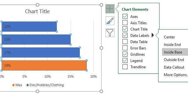
Add or remove data labels in a chart - support.microsoft.com Right-click the data series or data label to display more data for, and then click Format Data Labels. Click Label Options and under Label Contains, select the Values From Cells checkbox. When the Data Label Range dialog box appears, go back to the spreadsheet and select the range for which you want the cell values to display as data labels. How to Create a Bar Chart With Labels Above Bars in Excel In the Format Data Labels pane, under Label Options selected, set the Label Position to Inside Base. 10. Then, under Label Contains, check the Category Name option and uncheck the Value and Show Leader Lines options. 11. Next, while the labels are still selected, click on Text Options, and then click on the Textbox icon. 12. Showing percentages above bars on Excel column graph 0. The easy answer is you can edit the pivot table: -Right-click on the column showing series and goto pivot table options. -Click on Show values as an option. -Click on the percentage of grand total. -Enjoy :) Note: Although it will change the original values also to percentage.

Excel data labels above bar. How to Add Data Bars in Excel? - EDUCBA There are two kinds of Data Bars available in Excel. Select Gradient if you present both bar and numbers together or if you are showing only bars select Solid. You can change the color of the bar under Manage Rule and change the color there. How to Change Excel Chart Data Labels to Custom Values? First add data labels to the chart (Layout Ribbon > Data Labels) Define the new data label values in a bunch of cells, like this: Now, click on any data label. This will select "all" data labels. Now click once again. At this point excel will select only one data label. Go to Formula bar, press = and point to the cell where the data label ... data labels outside of bar graph | MrExcel Message Board #2 click on the bar you want to change-go to layout tab-data labels-outside end J johns99 Board Regular Joined Jun 11, 2013 Messages 210 Office Version 365 Platform Windows Oct 31, 2013 #3 I tried doing that originally and it doesn't give me the option for outside end M murphm03 Banned user Joined Dec 14, 2012 Messages 144 Oct 31, 2013 #4 Move data labels - support.microsoft.com Click any data label once to select all of them, or double-click a specific data label you want to move. Right-click the selection > Chart Elements > Data Labels arrow, and select the placement option you want. Different options are available for different chart types.

How to Show Labels Above Bar in a Horizontal Bar Chart It's not an uncommon scenario. You want to make your bar chart look a bit nicer (or different). You want to hide the dimension header, but you don't want the... How to Add Total Data Labels to the Excel Stacked Bar Chart For stacked bar charts, Excel 2010 allows you to add data labels only to the individual components of the stacked bar chart. The basic chart function does not allow you to add a total data label that accounts for the sum of the individual components. Fortunately, creating these labels manually is a fairly simply process. Add a DATA LABEL to ONE POINT on a chart in Excel Steps shown in the video above: Click on the chart line to add the data point to. All the data points will be highlighted. Click again on the single point that you want to add a data label to. Right-click and select ' Add data label ' This is the key step! Right-click again on the data point itself (not the label) and select ' Format data label '. Text Labels on a Horizontal Bar Chart in Excel - Peltier Tech On the Excel 2007 Chart Tools > Layout tab, click Axes, then Secondary Horizontal Axis, then Show Left to Right Axis. Now the chart has four axes. We want the Rating labels at the bottom of the chart, and we'll place the numerical axis at the top before we hide it. In turn, select the left and right vertical axes.

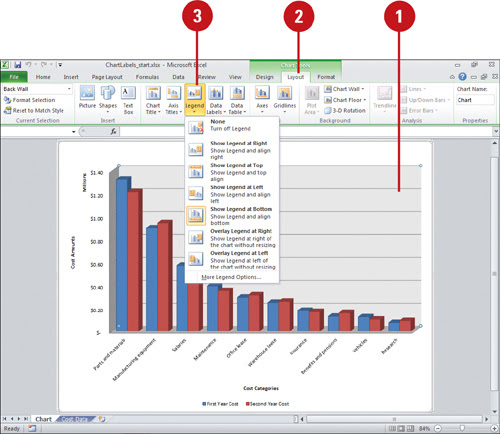
Custom Excel Chart Label Positions - My Online Training Hub Custom Excel Chart Label Positions - Setup. The source data table has an extra column for the 'Label' which calculates the maximum of the Actual and Target: The formatting of the Label series is set to 'No fill' and 'No line' making it invisible in the chart, hence the name 'ghost series': The Label Series uses the 'Value ... How do you put values over a simple bar chart in Excel? 1) Select cells A2:B5 2) Select "Insert" 3) Select the desired "Column" type graph 4) Click on the graph to make sure it is selected, then select "Layout" 5) Select "Data Labels" ("Outside End" was selected below.) how to add data labels above Line and Stacked Column chart Stacked Column Chart - Since there is more than one value per column, hence there is no concept of above in this case. Just consider one column on top of another. Lower column has no concept of above. In this case, you have to manually move them above the lower and other top columns. But in case of Line chart, you should get all the options. How to Customize Your Excel Pivot Chart Data Labels - dummies The Data Labels command on the Design tab's Add Chart Element menu in Excel allows you to label data markers with values from your pivot table. When you click the command button, Excel displays a menu with commands corresponding to locations for the data labels: None, Center, Left, Right, Above, and Below. None signifies that no data labels ...

Worth Data UK - LabelRIGHT Ultimate Bar Code Printing & Design Software for Windows

Format Data Labels in Excel- Instructions - TeachUcomp, Inc. To do this, click the "Format" tab within the "Chart Tools" contextual tab in the Ribbon. Then select the data labels to format from the "Chart Elements" drop-down in the "Current Selection" button group. Then click the "Format Selection" button that appears below the drop-down menu in the same area.

Excel Bar Chart with Vertical Line • My Online Training Hub

How to add or move data labels in Excel chart? - ExtendOffice 2. Then click the Chart Elements, and check Data Labels, then you can click the arrow to choose an option about the data labels in the sub menu. See screenshot: In Excel 2010 or 2007. 1. click on the chart to show the Layout tab in the Chart Tools group. See screenshot: 2. Then click Data Labels, and select one type of data labels as you need ...

How to Create a Stacked Bar Chart in Excel | Smartsheet

Add Data Bars in Excel (In Easy Steps) - Excel Easy To add data bars, execute the following steps. 1. Select a range. 2. On the Home tab, in the Styles group, click Conditional Formatting. 3. Click Data Bars and click a subtype. Result: Explanation: by default, the cell that holds the minimum value (0 if there are no negative values) has no data bar and the cell that holds the maximum value (95 ...

Use a bar chart in Excel to display YTD receipts and payments

Data Labels above bar chart - Excel Help Forum Re: Data Labels above bar chart You can link the data labels to other cells to display anything you want. Free addin to link labels to cells Attached Files 1142048b.xlsx‎ (21.0 KB, 18 views) Download Register To Reply Similar Threads Pie chart data labels By Duck1986 in forum Excel Charting & Pivots

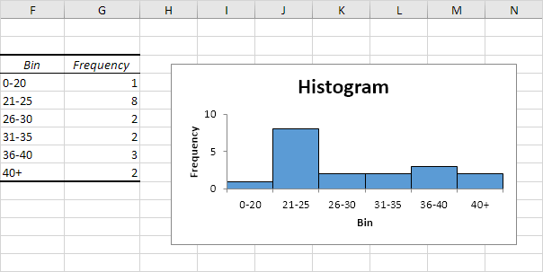
FREQUENCY function in Excel - Easy Excel Tutorial

How to add total labels to stacked column chart in Excel? Add total labels to stacked column chart in Excel Supposing you have the following table data. 1. Firstly, you can create a stacked column chart by selecting the data that you want to create a chart, and clicking Insert > Column, under 2-D Column to choose the stacked column. See screenshots: And now a stacked column chart has been built. 2.

Excel Graph Activities | Devpost

Axis Labels That Don't Block Plotted Data - Peltier Tech The charts below show the four positions for data labels in clustered column and bar charts. Center means in the center of the bars. Inside Base means inside the bar next to the base (bottom) of the bar (next to the axis). Inside End and Outside End mean inside and outside the far end of the bar. Stacked charts can't have Outside End labels ...

How to Create A Brain-Friendly Stacked Bar Chart in Excel

Excel Conditional Formatting Data Bars On the Ribbon, click the Home tab, and then in the Styles group, click Conditional Formatting. In the list of conditional formatting options, click Data Bars, and then click one of the Data Bar options -- Gradient Fill or Solid Fill. (see tips below) The selected cells now show Data Bars, along with the original numbers.

SQL Workbench/J User's Manual SQLWorkbench

How to Place Labels Directly Through Your Line Graph in Microsoft Excel Right-click on top of one of those circular data points. You'll see a pop-up window. Click on Add Data Labels. Your unformatted labels will appear to the right of each data point: Click just once on any of those data labels. You'll see little squares around each data point. Then, right-click on any of those data labels. You'll see a pop-up menu.

Directly Labeling Excel Charts - PolicyViz

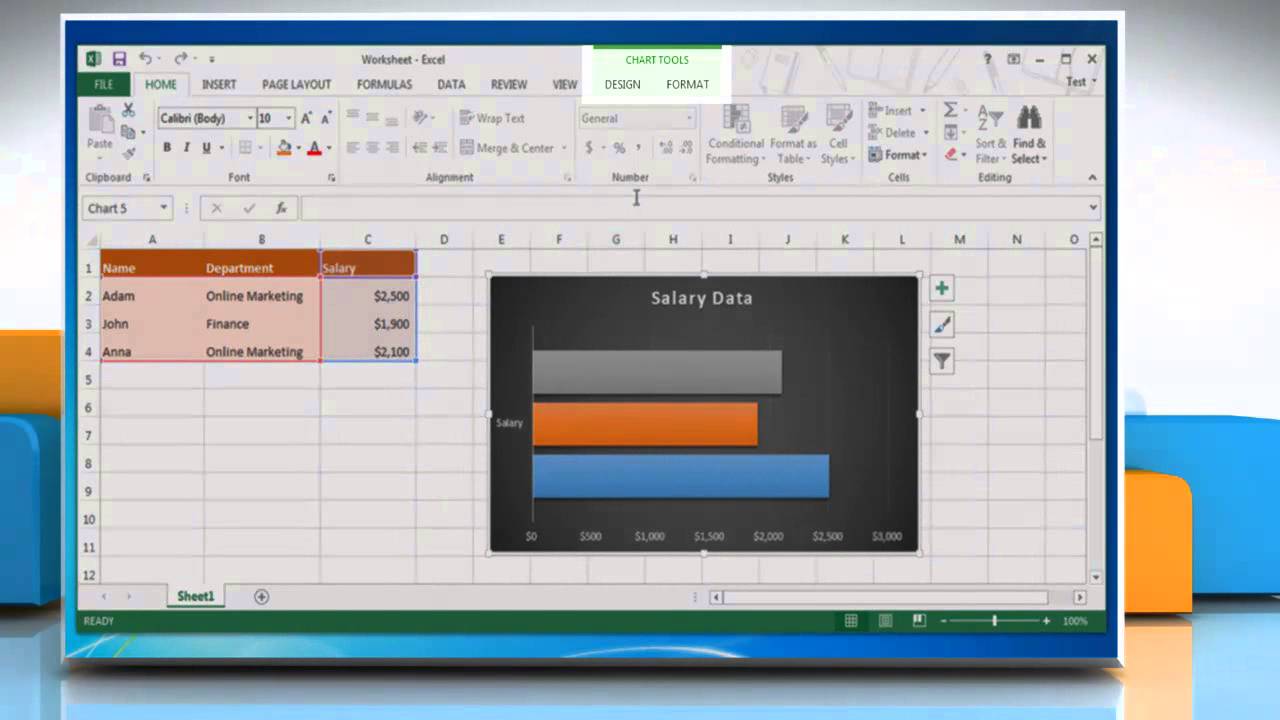
How to add data labels to a Column (Vertical Bar) Graph in ... - YouTube Get to know about easy steps to add data labels to a Column (Vertical Bar) Graph in Microsoft® Excel 2010 by watching this video.Content in this video is pro...

Quickly Create A Variable Width Column Chart In Excel

Showing percentages above bars on Excel column graph 0. The easy answer is you can edit the pivot table: -Right-click on the column showing series and goto pivot table options. -Click on Show values as an option. -Click on the percentage of grand total. -Enjoy :) Note: Although it will change the original values also to percentage.

How to Data Labels in a Bar Graph in Excel 2013 - YouTube

How to Create a Bar Chart With Labels Above Bars in Excel In the Format Data Labels pane, under Label Options selected, set the Label Position to Inside Base. 10. Then, under Label Contains, check the Category Name option and uncheck the Value and Show Leader Lines options. 11. Next, while the labels are still selected, click on Text Options, and then click on the Textbox icon. 12.