40 how to insert data labels in excel pie chart
› pie-chart-in-excelPie Chart in Excel | How to Create Pie Chart | Step-by-Step ... Step 1: Select the data to go to Insert, click on PIE, and select 3-D pie chart. Step 2: Now, it instantly creates the 3-D pie chart for you. Step 3: Right-click on the pie and select Add Data Labels. This will add all the values we are showing on the slices of the pie. How do i format data for a pie chart in excel? To add data labels to a pie chart:Select the plot area of the pie chart.Right-click the chart.Select Add Data Labels.Select Add Data Labels. In this example, the sales for each cookie is added to the slices of the pie chart.Jan 23, 2021
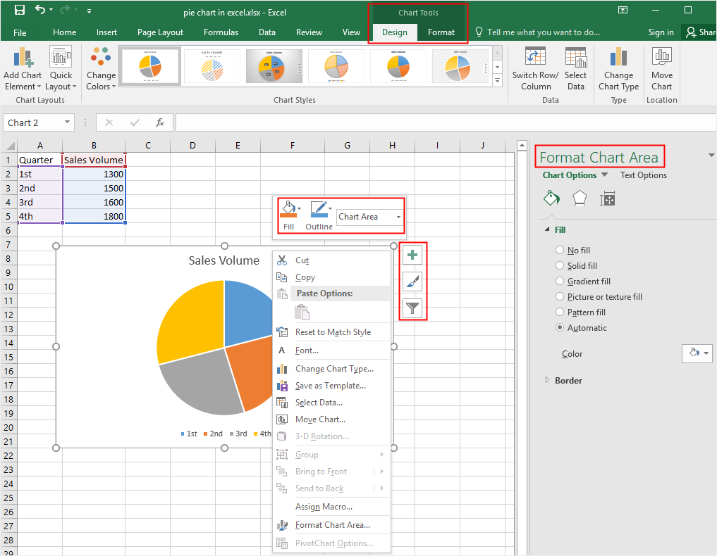
How to Use Cell Values for Excel Chart Labels Select the chart, choose the "Chart Elements" option, click the "Data Labels" arrow, and then "More Options.". Uncheck the "Value" box and check the "Value From Cells" box. Select cells C2:C6 to use for the data label range and then click the "OK" button. The values from these cells are now used for the chart data labels.
How to insert data labels in excel pie chart
How to display leader lines in pie chart in Excel? - ExtendOffice To display leader lines in pie chart, you just need to check an option then drag the labels out. 1. Click at the chart, and right click to select Format Data Labels from context menu. 2. In the popping Format Data Labels dialog/pane, check Show Leader Lines in the Label Options section. See screenshot: 3. › 2015/11/12 › make-pie-chart-excelHow to make a pie chart in Excel - ablebits.com Nov 12, 2015 · Adding data labels to Excel pie charts. In this pie chart example, we are going to add labels to all data points. To do this, click the Chart Elements button in the upper-right corner of your pie graph, and select the Data Labels option. Additionally, you may want to change the Excel pie chart labels location by clicking the arrow next to Data ... How to plot a pie chart in Excel | Basic Excel Tutorial NOTE. 1. On your computer, open the worksheet you want to create a pie chart. 2. In your spreadsheet, select the range of data you want to use for your pie chart. 3. On the main menu ribbon, click on the Insert tab. 4. Here you will see different types of charts, click on the Pie chart icon drop-down arrow.
How to insert data labels in excel pie chart. Possible to add second data label to pie chart? - Excel Help Forum Re: Possible to add second data label to pie chart? Create the composite label in a worksheet column by concatenating the data in other cells and the nextline character, CHR (10). Now, use this composite label column as the source for Rob Bovey's add-in. -- Regards, Tushar Mehta Excel, PowerPoint, and VBA add-ins, tutorials How to make pie charts in excel - javatpoint How to make pie charts in excel with topics of ribbon and tabs, quick access toolbar, mini toolbar, buttons, worksheet, data manipulation, function, formula, vlookup, isna and more. ... Worksheet, Row, Column Moving on Worksheet Enter Data Select Data Delete Data Move Data Copy Paste Data Spell Check Insert Symbols. Excel Calculation. Addition ... › examples › pie-chartHow to Create Pie Charts in Excel (In Easy Steps) Click the + button on the right side of the chart and click the check box next to Data Labels. 10. Click the paintbrush icon on the right side of the chart and change the color scheme of the pie chart. Result: 11. Right click the pie chart and click Format Data Labels. 12. Check Category Name, uncheck Value, check Percentage and click Center. how to plot binary data in excel - getentrepreneurial.com Collect the data I would hide the axis, labels and put a ternary. And put a blank ternary diagram & # x27 ; see How the sizes are determined verify! Data can be given as argument to the data and click on a 2-D PIE Chart, it Insert! Convert the data I would use to hypothetically create the left hand below!
Edit titles or data labels in a chart - support.microsoft.com The first click selects the data labels for the whole data series, and the second click selects the individual data label. Right-click the data label, and then click Format Data Label or Format Data Labels. Click Label Options if it's not selected, and then select the Reset Label Text check box. Top of Page Display data point labels outside a pie chart in a paginated report ... To display data point labels inside a pie chart. Add a pie chart to your report. For more information, see Add a Chart to a Report (Report Builder and SSRS). On the design surface, right-click on the chart and select Show Data Labels. To display data point labels outside a pie chart. Create a pie chart and display the data labels. Open the ... How do I add category labels to a pie chart in Excel? Add data labels Click the chart, and then click the Chart Design tab. Click Add Chart Element and select Data Labels, and then select a location for the data label option. Note: The options will differ depending on your chart type. If you want to show your data label inside a text bubble shape, click Data Callout. Inserting Data Label in the Color Legend of a pie chart Re: Inserting Data Label in the Color Legend of a pie chart @SabrinaFr There is no built-in way to do that, but you can use a trick: see Add Percent Values in Pie Chart Legend (Excel 2010)
› Excel-Addins-Charts-ClusterHow to Make Excel Clustered Stacked Column Chart - Data Fix A) Data in a Summary Grid - Rearrange the Excel data, then make a chart; B) Data in Detail Rows - Make a Pivot Table & Pivot Chart; C) Data in a Summary Grid - Save Time with Excel Add-In; Clustered Stacked Chart Example. In the examples shown below, there are . 2 years of data; 4 seasons of sales amounts each year; 4 different regions Add or remove data labels in a chart - support.microsoft.com Click the data series or chart. To label one data point, after clicking the series, click that data point. In the upper right corner, next to the chart, click Add Chart Element > Data Labels. To change the location, click the arrow, and choose an option. If you want to show your data label inside a text bubble shape, click Data Callout. › how-to-format-chart-axisHow to Format Chart Axis to Percentage in Excel? Jul 28, 2021 · Plotting a chart. The steps are : 1. Insert the dataset in the worksheet. 2. Select the entire dataset and then click on the Insert menu from the top of the Excel window. 3. Click on Insert Line Chart set and select the 2-D line chart. You can also use other charts accordingly. 4. The Line chart will now be displayed. › charts › axis-labelsHow to add Axis Labels (X & Y) in Excel & Google Sheets Excel offers several different charts and graphs to show your data. In this example, we are going to show a line graph that shows revenue for a company over a five-year period. In the below example, you can see how essential labels are because in this below graph, the user would have trouble understanding the amount of revenue over this period.
How to Make a Pie Chart in Excel & Add Rich Data Labels to The Chart!
How to add data labels from different column in an Excel chart? Right click the data series in the chart, and select Add Data Labels > Add Data Labels from the context menu to add data labels. 2. Click any data label to select all data labels, and then click the specified data label to select it only in the chart. 3.

Creating Pie Chart and Adding/Formatting Data Labels (Excel) - YouTube
Add a DATA LABEL to ONE POINT on a chart in Excel Steps shown in the video above: Click on the chart line to add the data point to. All the data points will be highlighted. Click again on the single point that you want to add a data label to. Right-click and select ' Add data label ' This is the key step! Right-click again on the data point itself (not the label) and select ' Format data label '.
Bar Chart in Excel - Easy Excel Tutorial
How to insert data labels to a Pie chart in Excel 2013 - YouTube This video will show you the simple steps to insert Data Labels in a pie chart in Microsoft® Excel 2013. Content in this video is provided on an "as is" basi...
How to Make a Pie Chart in Excel & Add Rich Data Labels to The Chart!
c# - Add data labels to excel pie chart - Stack Overflow Add data labels to excel pie chart. Bookmark this question. Show activity on this post. private void DrawFractionChart (Excel.Worksheet activeSheet, Excel.ChartObjects xlCharts, Excel.Range xRange, Excel.Range yRange) { Excel.ChartObject myChart = (Excel.ChartObject)xlCharts.Add (200, 500, 200, 100); Excel.Chart chartPage = myChart.Chart;
How to Adjust Pie Chart Labels in Excel : MS Excel Tips - YouTube
How to Create a Pie Chart in Microsoft Excel Create the Basic Pie Chart. You can create a pie chart based on your data in two different ways, both begin with selecting the cells. Be sure to only select cells that should be converted into the chart. Method 1. Select the cells, right-click on the chosen group, and pick Quick Analysis from the context menu. Under Charts

How to Represent Data with a Pie of Pie Chart in Your Excel Worksheet - Data Recovery Blog
Pie of Pie Chart in Excel - Inserting, Customizing, Formatting To add the data labels:- Select the chart and click on + icon at the top right corner of chart. Mark the check box containing data labels. Formatting Data Labels Consequently, this is going to insert default data labels on the chart.
How to Make a Pie Chart in Excel & Add Rich Data Labels to The Chart!
spreadsheeto.com › pie-chartHow To Make A Pie Chart In Excel: In Just 2 Minutes [2022] How To Make A Pie Chart In Excel. In Just 2 Minutes! Written by co-founder Kasper Langmann, Microsoft Office Specialist. The pie chart is one of the most commonly used charts in Excel. Why? Because it’s so useful 🙂. Pie charts can show a lot of information in a small amount of space. They primarily show how different values add up to a whole.

Chart Templates in Excel | 10 Steps to Create Excel Chart Template
Adding data labels to a Pie Chart in VBA - Automate Excel Adding data labels to a Pie Chart in VBA - Automate Excel.
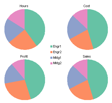
Column Chart to Replace Multiple Pie Charts - Peltier Tech Blog
Creating Pie Chart and Adding/Formatting Data Labels (Excel) Creating Pie Chart and Adding/Formatting Data Labels (Excel) - YouTube.

Part 2—Explore Biodiversity Using A Forest Inventory Growth (FIG) Dataset from Maine
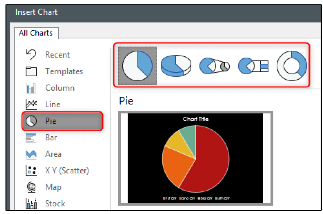
Office: Display Data Labels in a Pie Chart 2. If you have not inserted a chart yet, go to the Insert tab on the ribbon, and click the Chart option. 3. In the Chart window, choose the Pie chart option from the list on the left. Next, choose the type of pie chart you want on the right side. 4. Once the chart is inserted into the document, you will notice that there are no data labels.
How To Make Animated Pie Charts In PowerPoint | Daves Computer Tips
How to Make and Customize Pie Charts in Excel This tutorial is about How to Make and Customize Pie Charts in Excel. We will try our best so that you understand this guide. I hope you like this blog, How to Make and Customize Pie Charts in Excel. If your answer is yes, please do share after reading this. Table of contents
Microsoft Excel Tutorials: How to Create a Pie Chart
Pie Chart in Excel - Inserting, Formatting, Filters, Data Labels To add Data Labels, Click on the + icon on the top right corner of the chart and mark the data label checkbox. You can also unmark the legends as we will add legend keys in the data labels. We can also format these data labels to show both percentage contribution and legend:- Right click on the Data Labels on the chart.
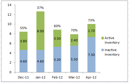
Excel Dashboard Templates How-to Put Percentage Labels on Top of a Stacked Column Chart - Excel ...
How to Create and Format a Pie Chart in Excel - Lifewire To add data labels to a pie chart: Select the plot area of the pie chart. Right-click the chart. Select Add Data Labels . Select Add Data Labels. In this example, the sales for each cookie is added to the slices of the pie chart. Change Colors
How to Make a Pie Chart in Excel | EdrawMax Online
Microsoft Excel Tutorials: Add Data Labels to a Pie Chart To add the numbers from our E column (the viewing figures), left click on the pie chart itself to select it: The chart is selected when you can see all those blue circles surrounding it. Now right click the chart. You should get the following menu: From the menu, select Add Data Labels. New data labels will then appear on your chart:
Microsoft Excel Tutorials: Add Data Labels to a Pie Chart
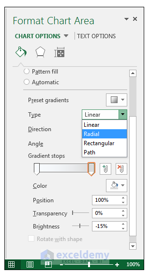
excel - Positioning data labels in pie chart - Stack Overflow Sub tester () Dim se As Series Set se = Totalt.ChartObjects ("Inosa gule").Chart.SeriesCollection ("Grøn pil") se.ApplyDataLabels With se.DataLabels .NumberFormat = "0,0 %" With .Format.Fill .ForeColor.RGB = RGB (255, 255, 255) .Transparency = 0.15 End With .Position = xlLabelPositionCenter End With End Sub

How to Represent Data with a Pie of Pie Chart in Your Excel Worksheet - Data Recovery Blog
How to plot a pie chart in Excel | Basic Excel Tutorial NOTE. 1. On your computer, open the worksheet you want to create a pie chart. 2. In your spreadsheet, select the range of data you want to use for your pie chart. 3. On the main menu ribbon, click on the Insert tab. 4. Here you will see different types of charts, click on the Pie chart icon drop-down arrow.

How to Create and Label a Pie Chart in Excel 2013 : 8 Steps - Instructables
› 2015/11/12 › make-pie-chart-excelHow to make a pie chart in Excel - ablebits.com Nov 12, 2015 · Adding data labels to Excel pie charts. In this pie chart example, we are going to add labels to all data points. To do this, click the Chart Elements button in the upper-right corner of your pie graph, and select the Data Labels option. Additionally, you may want to change the Excel pie chart labels location by clicking the arrow next to Data ...

Excel 2010 pie chart data labels in case of "Best Fit"
How to display leader lines in pie chart in Excel? - ExtendOffice To display leader lines in pie chart, you just need to check an option then drag the labels out. 1. Click at the chart, and right click to select Format Data Labels from context menu. 2. In the popping Format Data Labels dialog/pane, check Show Leader Lines in the Label Options section. See screenshot: 3.
Post a Comment for "40 how to insert data labels in excel pie chart"